my alt text

Why Open the Black Box?

Since the dawn of time, deep learning models have been puzzling theoreticians as to why they work so well. With the large amounts of parameters they have, the fact that they seem to generalize well is a confounding one. Of course getting them to work well is often easier said then done. Today’s models typically have more buttons and switches to fiddle with than an airplane cockpit. And much like an airplane, flipping the wrong set of switches is likely to end in a crash and burn scenario. Its definitely true that some good general machine learning knowledge can help in setting these parameters, but there are many times where it seems the only thing we have to guide us is our shaky intuition.

A good theory can often serve as an highly effective guide for practitioners. While understanding the theory of why deep learning models work may not completely eliminate all the knobs we need to set, it would definitely make many choices much easier. Its no surprise that there has been some theory work on trying to understand deep learning models.

Looking at the Black Box Using Information Theory

One that has recently gotten some attention (in the form of articles from mainstream press such as Quanta, as well as praise from Geoffrey Hinton himself) has been the work of Naftali Tishby’s lab, on providing an information theory based explanation as to why these models can generalize. Most of the excitement revolves around the work titled “Opening the Black Box of Deep Neural Networks via Information” however the main theoretic arguments were actually presented two years ago, in 2015.

Since some of the conclusions above are empirical, some caution should be taken before fully accepting its conclusions (indeed a currently under review paper in ICLR 2018 gives results that contradict the above paper¹), however the theory behind it is incredibly appealing, and holds a lot of value in itself. In this post I hope to give an overview of the theory, the main points behind it, and what it could possibly mean for the future of deep learning. At this point I will proceed with describing the preliminaries to understanding Tishby’s information theory-deep learning connection: Rate Distortion Theory, and the Information Bottleneck principle. The post assumes you have a grasp on the basic ideas of deep learning, and an understanding of basic concepts from information theory such entropy and mutual information (this concept is important!). This post is a great introduction to these concepts if you need a hand.

What does information theory have to do with deep learning?

What exactly is the connection between information theory (IT) and deep learning (DL)? Rather than jump right into connection between the two it actually helps to first understand the Information Bottleneck (IB) principle. As we will see, once we understand IB, the connection between IT and DL arises quite naturally. The main purpose of IB is to answer the following question: “How do we define what information in relevant, in a rigorous way?” This seems rather counter-intuitive, as the ‘relevancy’ of information seems rather subjective. Information theory as laid out by Claude Shannon omits any notion of ‘meaning’ in the information, and without meaning, how can we possibly measure relevancy?

Rate Distortion Theory

Information theory does hold one possible answer to the question of relevancy however, in the form of lossy compression. The goal of lossy compression is to find the ‘most compressed’ representation possible for our set of input data $X$ such that we don’t lose too much information about our original data $X$. Our relevant information would thus be the information preserved in the compressed version of $X$. Rate Distortion Theory provides a clear formalization for these concepts.

Defining Compression The first thing we need to to formalize is how the ‘compression’ is actually done. We can formally think of compression as defining a (possibly stochastic) function that maps an element $x \in X$ to its corresponding compressed representation (sometimes called the ‘codeword’ for $x$). We will refer to the set of codewords of $X$ as $T$, with an arbitrary element of $T$ being denoted as $t$ This map is implicitly defined through the probability distribution $p(t|x)$, so by defining the distribution $p(t|x)$ we will have defined our method of compression/assignment of codewords.

The diagram below gives a visual representation of this compression (for a deterministic $p(t|x)$, which is what we will have with most neural networks):

my alt text

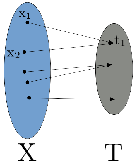
As you can see, there may be many elements of $X$ that map to the same $t \in T$.

Measuring Compression We now need a good mathematical way to measure how ‘compressed’ our representation (decided by $p(t|x)$) is. One natural way to measure how much we have compressed the set of codewords is to measure how much information a codeword contains (on average). This can be done of course by using the entropy rate of T². The rate of T can be made arbitrarily large however simply by packing redundant information in the codewords. What we are interested in measuring is the best rate we can achieve for a certain type of encoding (recall, this is defined by $p(t|x)$). It turns out the mutual information between $X$ and $T$ (denoted $I(X;T)$ gives a lower bound on the rate of $T$, thus we can use $I(X;T)$ as a stand in for ‘the best rate achieved for encoding $p(t|x)$’ and thus as a measure of how ‘compressed’ representation $T$ is³ The smaller $I(X;T)$ the more compressed a representation $T$ is of $X$ (this should make intuitive sense, smaller $I(X;T)$ means $T$ holds less information about $X$, which is what we would expect as our representation gets more compressed). Of course, higher values of mutual information indicate a less compressed representation.

Losing Information One more thing we need to formalize: we need to define how much information loss is too much information loss, and more particularly, what constitutes as information loss. We do this by defining a distortion function $d(x,t)$, which takes in an element of $X$ and $T$ and outputs a single value indicating how different (ie distorted) $x$ and $t$ are. The exact function is arbitrary and must be picked on a per task basis (if our data was images, we would probably want a different distortion measure then if we were using something like text data). Example distortion functions include squared difference or Hamming distance between the input $x$ and $t$, but there are many possible distortion functions that can be defined.

Now that we have a distortion function, we would like to be able to measure how much information is lost when using the encoding defined by $p(t|x)$. For this we can use the expected distortion $D(p)$:

$D(p)= \sum_{x,t} p(x,t)d(x,t)$

A smaller value of $D(p)$ can be reached by making sure $x,t$ pairs with high joint probability (remember, $p(x,t)=p(t|x)p(x)$) have a low value of $d(x,t)$.

We can define how much information loss is too much by defining a threshold value $D^*$, and refusing to use any compression method (ie a specific set of representations $T$) whose expected distortion $D(p) > D^*$.

Rate Distortion Curves With all this in place we can now answer the golden question: What’s the most we can possibly compress an input (equivalently, how low can we get the rate of $T$) if we are allowed to distort the input up to threshold $D^*$? Note that we ask this question without regard to the compression method. This is a theoretical limit, the best that we can (or ever will) do. The answer is deceptively simple, the best (lowest) rate we can get is equal to the mutual information under the best possible compression method $p(t|x)$. This value is described through the rate distortion function, which takes in a threshold $D^*$ and returns the rate of the best possible $p(t|x)$ we can use:

$R(D^*) = \min_{p(t|x):D(p) \leq D^*} I(X;T)$

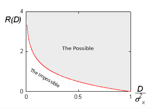
We can look at this problem as a constrained optimization problem, where we wish to find a $p(t|x)$ that minimize $I(T;X)$, with a constraint on $D(p)$ (this is typically turned into an unconstrained problem by using Lagrangian multipliers). Given we know $P(X)$, the above optimization problem can, in practice, be solved!⁴ Note that for each value of $D^*$ we get a different value of best possible rate, $R$. We can plot $R$ as a function of $D^*$ to get what is called the rate distortion curve. An example Rate Distortion Curve (taken from the Wikipedia article) is shown below. This curve represents the optimal values of $R$, any values above the curve are sub optimal (meaning the representations $T$ are sub optimal), any values below the curve are theoretically impossible to achieve. This idea of a rate distortion curve will be central later on, so make sure you are comfortable with it. One of the important things to note on the curve is that there is a constant theoretical tug of war between rate and distortion. You want to lower the rate? You’ll inevitably need to add more distortion. Want to lower amount of distortion? Well your rate is going to have to go up.

no image

This is the main gist of of RDT, the question is can it be used to define what information in our signal is relevant? Alas, the answer is no. The biggest problem is that the distortion function itself must be defined. By defining the distortion function, we are essentially defining what information is relevant in the signal $X$, which is the very thing we are trying to find out! It’s clear that some of the ideas of RDT can be useful for defining relevant information, however we need to be a bit more clever in terms of how we define relevancy.

TL;DR Rate Distortion Theory Here are the main takeaways from Rate Distortion Theory:

Mutual Information $I(X;T)$ can be seen as measuring the amount of compression
There’s always a tug-a-war between our rate and distortion values
With the pairs of optimal rate and distortion values, we can define a curve called the rate distortion curve
We have to provide a distortion measure, and because of this, Rate Distortion Theory doesn’t serve our mission of defining information relevancy in a rigorous way.

The Information Bottleneck Method

The information bottleneck principle (IB) is quite similar to RDT, with some key differences. Instead of defining relevance directly through the set of codewords $T$, IB instead defines relevance through another variable $Y$. That is, given an input signal $X$, we would like to find a compressed representation of $X$ (again this set of codewords $T$) such that $T$ preserves as much information about the output signal $Y$ as possible. Like RDT, we still want to obtain as compressed a representation of $X$ as possible (ie we still want to minimize $I(X;T)$, however now our constraint is different. Our goal in IB is to choose a representation $T$ (which, like RDT, is still defined by $p(t|x)$) which preserves as much information about $Y$ as possible. How do we measure how much information about $Y$ the representations $T$ have? Mutual information of course! Rather than constraining how much distortion occurs like in RDT, in IB we constrain how much information about $Y$ we are willing to lose by compressing $X$ into $T$. We do this by indicating the minimum value of $I(T;Y)$ (denoted as $I^*$) we are willing to have in a representation $T$. This leads to the optimization problem:

$\min_{p(t|x):I(T;Y) \geq I^*} I(X;T)$

Like RDT, this optimization problem can also be solved (given we know $P(X,Y)$).

The Bottleneck In order to get a good representation $T$, we must ‘squeeze out’ any information in $X$ that is irrelevant to $Y$, leaving us only the parts of $X$ relevant to $Y$. This is the bottleneck in the information bottleneck principle. For each value of $I(T;Y)$ there is a corresponding minimal value of $I(X;T)$. So just like in RDT we can define a sort of rate distortion curve of corresponding optimal $I(T;Y)$, $I(X;T)$ pairs (to avoid confusion, I will refer to this as the rate-information curve). Just like in a rate distortion curve, this curve defines the optimal values, this time with impossible values laying above the curve, and sub optimal values below the curve. Note that just like in RDT, there is always tug of war between the rate value $I(X;T)$, and the information value $I(Y;T)$. It is important to realize that this curve is defined solely by the distribution $P(X,Y)$, since given this distribution we can solve the above optimization problem. The set of all points (all possible pairs of $I(X;T), I(T;Y)$ values, both optimal and sub-optimal) form what is called the information plane. As we shall see, analyzing deep learning models with respect to the information plane will be a key insight the IB principle brings to deep learning.

Deep Learning and the Information Bottleneck

We now come to the whole purpose of this write up, the IB connection with deep learning. As you might have been noticing, IB sort of ‘smells’ like deep learning. In particular, you may have noticed these following analogs: $X$=Inputs, $T$=Hidden Layers, $Y$=Outputs. Indeed you would be correct here! In deep learning we can think of the set of codewords $T$ as being the representations output by one of the hidden layers of the network. Of course in deep learning, we typically have many hidden layers (let’s say we have $k$ here), and thus we have many sets of codewords for $X$. For notational purposes, let $T_i$ indicate the outputs for the $ith$ hidden layer . Other than the fact that we have $k$ sets of codewords, we can treat everything pretty much the same as in IB theory. With IB we can measure how good the representation of each layer is by looking at $I(Y;T_i)$. We can additionally see how much we have compressed the input $X$ at the $ith$ layer by looking at $I(X;T_i)$.

Losing Information An important fact to note is that each time we go through a layer of our network, we have no way to obtain extra information about $Y$. All the information that we know about $Y$ comes from $X$. Its not possible for new information about $Y$ to magically appear simply because we compress $X$ into a new representation $T_i$. So each time we obtain a new representation $T_i$ by going through the $ith$ hidden layer, we lose a little information about $Y$ (at the very best we lose no information on $Y$). This can be described through the following inequality (called the Data Processing Inequality) for all $j>i$:

$I(Y;X) \geq I(T_i;Y) \geq I(T_j;Y) \geq I(Y';Y)$

$Y’$ here indicates the outputs of our network. Note that with each layer, we have an associated $I(X;T)$ and $I(T;Y)$$ pair, which means we can thus plot it as a point on the information curve.

Learning by forgetting You may be scratching your head at this apparent contradiction. Doesn’t having multiple layers help us in deep learning? Why do we want to add more layers if they simply make us lose information about $Y$?

First recall that the curve (and thus all values of $I(X;T)$ and $I(T;Y)$) is defined solely by the distribution $P(X,Y)$, a distribution that we do not have access to. However we do have access to a set of $n$ samples, $S$ from the true distribution. This of course, is our training set. With $S$ we can make an empirical estimate of the joint distribution, $\hat{P}(X,Y)$ by using some maximum likelihood method. With this empirical distribution, we can calculate the empirical mutual information values, $\hat{I}(X;T)$ and $\hat{I}(T;Y)$. How far off our empirical estimate $\hat{I}(T;Y)$ is from $I(T;Y)$ is proven to have the following bounds (similar bounds are proven for $\hat{I}(X;T)$ as well):

$I(T;Y) \leq \hat{I}(T;Y) + O\Big(\frac{|T|*|Y|}{\sqrt{n}}\Big)$

Where $|T|$ is the cardinality of $T$, which is approximately equal to $2^{I(X;T)}$. So the tightness of the bound depends on how compressed $T$ is! As $T$ becomes more compressed, $I(X;T)$ becomes smaller, meaning the bound above becomes tighter, meaning our empirical estimate $\hat{I}(T;Y)$ is more likely to be closer to the true value of $I(T;Y)$.

But why is this important? We don’t really care about estimating $I(T;Y)$ in the end, what we really care about is minimizing the generalization error (that is, minimize the probability of a misclassification on an arbitrary instance from the test set). Surprisingly, it turns out that $I(T;Y)$ can actually act as a stand in for the generalization error!

For a classification problem, if we always choose a class $y$ by picking the class that maximizes the likelihood of $y$ with respect to $T$ (that is, maximizes the probability $P(t|y)$), then $I(T;Y)$ actually (roughly⁵) forms a lower bound on the negative log probability of error. Thus $I(T;Y)$ can be used as a proxy for generalization performance! The higher $I(T;Y)$ is, the better our system generalizes. The lower $I(X;T)$ is, the tighter the bound is between our empirical estimate $\hat{I}(T;Y)$ and the true generalization performance $I(T;Y)$. As said in Tishby and Zaslavsky, 2015:

“The hidden layers must compress the input in order to reach a point where the worst case generalization performance error is tolerable”.

Looking at Networks in the Information Plane

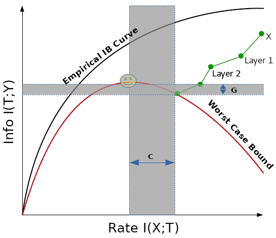
With this all set up, we can now think of our network as indicating a point somewhere on the information plane (that is, with respect to $I(T;Y)$ and $I(X;T)$). The poorly drawn chart below gives a picture of this. The locations of our network on the information plane are indicated by the green arrows. Of course, we start at a point (just the input $X$) with less compression, and more information about $Y$ (since $X$ contains all the information about $Y$ that we can ever get). As we add hidden layers our representation becomes more and more compressed, and we lose information about $Y$. With our training data we can estimate an empirical information curve (represented by the black curve) as well as a worst case bound for our estimated value of $I(T;Y)$ (indicated by the red curve).

One important thing to remember about the chart is the only thing that is really true with respect to the true distribution $P(X,Y)$ is the red curve! The rest of the curves, including the location of our network on the information plane, are simply empirical estimates. However, we can take solace in knowing that we will never go below the red curve. Ideally we would like to end up at the maximum value of the red curve, as this indicates the best worst case scenario for us, giving us the location on the information plane where the generalization bound is tightest. We can refer to this point as $R^*$. On the graph below, the point is indicated via the standard smiley face notation. Of course, there is no reason you should expect SGD to take us to the optimal point. How far we are from $R^*$ on the $I(X;T)$ axis is called the complexity gap, $C$. It indicates how much more we could have compressed our inputs. How far we are from $R^*$ in terms of $I(T;Y)$ is called the generalization gap, $G$. It indicates how much more information about $Y$ we could have stuffed into our representations.

no image

Concluding Thoughts

By looking through the lens of information theory we have developed a theoretically well motivated framework that provides us with another way of thinking about neural networks. (in terms of compression and information relevancy) What does this mean for the future? The theoretical tools presented here could possibly motivate a whole wide array of optimization techniques whose goal is to reach the elusive $R^*$. The whole concept of compression leading to better generalization might motivate theoretical analysis into why techniques such as dropout (and other mysterious techniques) work. The possibilities are, as they say, countably infinite. The next interesting step would be to try to analyze real networks in the information plane, which is what “Opening the Black Box of Deep Neural Networks via Information” does. The next post will discuss these results, the contradictory results reported in a new ICLR submission, the implications of these results, as well as some of the practical challenges of analyzing networks in the information plane.

One more concluding thought…

One last thing to note before you go. Above I said that $I(T;Y)$ can form a bound on generalization error if we use a decision rule which selects the class $y$ that maximizes the likelihood of $y$. For networks that train on cross entropy error (most networks that perform multi-class classification do), the decision rule typically employed is to select the class the maximizes data likelihood (ie. maximizes the probability $p(y|t)$). This is the same as maximizing $p(t|y)$ if our distribution of class labels $P(Y)$ is uniform, though this often is never the case. So is this a cause for concern? I don’t really know, which is why I am putting it here. Intuitively switching the decision rules from maximum likelihood to MAP seems like it shouldn’t have to much of an impact. I haven’t heard any discussions about this, so it would be nice if future work could possibly address this issue (if its an issue). Feel free to leave a comment if you have any insights into this.

References

O. Shamir, S. Sabato, and N. Tishby. “Learning and generalization with the information bottleneck.” ALT. Vol 8. 2008.
R. Shwartz-Ziv and N. Tishby. “Opening the Black Box of Deep Neural Networks via Information”. ArXiv. https://arxiv.org/abs/1703.00810. April 2017.
N. Tishby and N. Zaslavsky. “Deep Learning and the Information Bottleneck Principle”. arXiv. https://arxiv.org/abs/1503.02406. March 2015.
N. Tishby, F.C. Pereira, and W. Bialek. “The information bottleneck method”. arXiv. https://arxiv.org/abs/physics/0004057. 1999.

For those interested, a rebuttal from Tishby and Shwartz-Ziv has been posted on the given link ↩
There is a slight difference between the entropy rate and just plain old entropy, the difference however is not important here ↩
It actually turns out that $I(X;T)$ is even better than a lower on the ‘best achievable rate’… the two are equivalent! ↩
The problem can be solved by an alternating algorithm called the Blahut-Arimoto algorithm, a similar method is used to solve the IB equations ↩
See (Shamir, Sabato, and Tishby, 2008) for the proof of this bound, as well as the other generalization bounds for IB ↩